Understanding the binomial distribution in business and banking
The binomial distribution is a fundamental concept in probability and statistics, widely used in various fields, including business, finance, and quality control. It provides a model for predicting the number of successes in a fixed number of trials, each with the same probability of success. Understanding the binomial distribution is crucial for making informed decisions and accurately assessing risks in uncertain scenarios. In this article, we will learn about the key factors that define the binomial distribution, explore its formula, and examine practical applications in business and banking.

What is binomial distribution?
The binomial distribution is a probability distribution that summarises the likelihood that a value will take one of two independent states under a given number of parameters. It describes the number of successes in a fixed number of trials, each with the same probability of success.
Understanding binomial distribution
The term “binomial” in binomial distribution reflects two possible outcomes—successes and attempts. In the binomial context, each outcome is only meaningful when paired with the other.
Binomial distribution is a key discrete probability distribution in statistics, differing from continuous distributions like the normal distribution. It focuses on two states, typically represented by 1 (success) or 0 (failure), across a given number of trials. The binomial distribution calculates the likelihood of observing a specified number of successes, xxx, in a set of nnn trials, given a constant probability of success, ppp, for each trial.
This distribution summarizes the behavior of repeated trials or observations where each has the same chance of achieving a particular outcome. By doing so, the binomial distribution effectively models the probability of obtaining a specific count of successful outcomes within a defined number of trials.
Properties of binomial distribution
The binomial distribution has several distinct properties that make it suitable for modeling situations with two possible outcomes. Here are the key characteristics:
Two possible outcomes:
Each trial in a binomial distribution has two possible outcomes, commonly labeled as success or failure. These outcomes are often represented by binary values, such as true/false, yes/no, or 1/0.
Fixed number of trials:
In a binomial distribution, there is a fixed number of trials, denoted as nnn. Each trial is repeated a set number of times, which means the distribution focuses on a specific number of attempts or experiments.
Constant probability of success:
The probability of success (often denoted by ppp) is the same for each trial. This constancy ensures that each trial is identical in terms of its chance of resulting in a success or failure, making the model reliable across all trials.
Counting successes:
The binomial distribution is concerned with the number of successes observed across the nnn trials. It does not account for failures directly; rather, it focuses on the total count of successes over the fixed number of trials.
Independence of trials:
Each trial is independent, meaning that the outcome of one trial does not influence the outcome of another. This independence is a crucial requirement, ensuring that each trial’s result is unaffected by any previous trial’s outcome.
These properties make the binomial distribution a powerful tool in statistics, particularly in scenarios where events occur in a controlled and repeatable manner with clearly defined success probabilities and independence conditions.
Key factors of the binomial distribution
To understand the binomial distribution fully, it’s essential to grasp the key factors that define it:
Number of trials (n)
The number of trials (n) is the total count of independent events being analysed. For instance, a bank might process 100 loan applications within a month. This number is fixed and crucial for binomial probability calculations.
Probability of success (p)
The probability of success (p) represents the likelihood that any single trial will succeed. If historically, 70% of loan applications are approved, p would be 0.70. This probability remains constant across all trials.
Number of successes (k)
The number of successes (k) indicates the number of trials that resulted in a successful outcome. For example, if 70 out of 100 loan applications are approved, k is 70. The binomial distribution helps calculate the probability of getting exactly k successes out of n trials.
Probability of failure (1-p)
The probability of failure (1-p) is the likelihood that a single trial will result in failure. It is simply 1 minus the probability of success. Using the earlier example, if the success rate is 70% (p = 0.70), then the failure rate is 30% (1-p = 0.30).

Example of Binomial Distribution
The binomial distribution helps calculate probabilities by combining the principles of permutations and likelihood. It considers the probability of success to the power of the number of successes and the probability of failure to the power of the number of failures, multiplied by the number of ways these successes can occur within the trials.
For instance, imagine a casino introducing a new betting game based on the number of heads obtained in several coin flips. A participant decides to wager $10 on getting exactly six heads out of 20 flips. To find out the likelihood of this happening, the participant uses the binomial distribution formula.
The calculation is as follows: 20!6!×(20−6)! * (0.50)6* (0.50)14
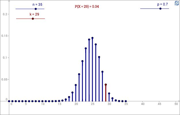
This results in a probability of approximately 0.0369, or 3.7%. Given that the expected number of heads is 10, this bet is statistically disadvantageous. A graph illustrating this distribution would show the probability peak at 10 heads, with six heads appearing towards the less likely left tail, colored in red to indicate its lower probability compared to outcomes of seven through thirteen heads.
Applications in banking and business
The binomial distribution is a powerful tool in banking and business, helping to predict outcomes and make informed decisions. Here are some key applications:
Risk management
Banks use the binomial distribution to assess the probability of loan defaults. By knowing the historical default rate, they can estimate the likelihood of a certain number of defaults in a portfolio of loans. This helps in managing credit risk and setting aside appropriate reserves. For example, if a bank has a default rate of 5%, it can predict the probability of having 10 or more defaults out of 200 loans issued.
Marketing campaigns
Businesses apply the binomial distribution to forecast the success of marketing campaigns. For instance, if a company knows the response rate to previous campaigns is 20%, it can predict the number of positive responses to a new campaign. This aids in budget allocation and strategy planning by estimating the return on investment and planning resources accordingly.
Quality control
In manufacturing, the binomial distribution is used to monitor product quality. By understanding the defect rate, companies can predict the number of defective items in a batch and take corrective actions to maintain quality standards. For example, if a factory produces 1,000 items with a 2% defect rate, the binomial distribution can predict how many defective items will likely be found in a random sample.
Employee performance
Companies can use the binomial distribution to evaluate employee performance. For instance, if a sales team has a historical success rate for closing deals at 30%, the distribution helps predict the number of deals closed in a given period. This information can inform performance reviews and incentive programmes, helping managers set realistic targets and reward high performers.
Financial forecasting
Businesses use the binomial distribution to model financial scenarios. For example, it helps forecast cash flows based on the probability of receiving payments from clients, aiding in liquidity management and financial planning. If a business has a 90% chance of receiving payment from each of its 50 clients, the binomial distribution can estimate the expected number of payments and the associated cash flow.

Relationship with other distributions
The binomial distribution is interconnected with other statistical distributions, each serving different purposes in business analysis:
Bernoulli distribution
The Bernoulli distribution is a special case of the binomial distribution with a single trial (n = 1). It models the probability of success in one trial, making it foundational for understanding the binomial distribution. In business, it helps in scenarios where a single event outcome is of interest, such as the success of a single marketing call or the outcome of a one-time product test.
Normal distribution
For large sample sizes, the binomial distribution approximates the normal distribution due to the Central Limit Theorem. This is useful in business for simplifying calculations and making inferences about large datasets. For instance, predicting overall sales from numerous transactions becomes easier by approximating the binomial distribution to a normal distribution, which is more manageable and interpretable.
Poisson distribution
When dealing with rare events and many trials with a small probability of success, the binomial distribution approximates the Poisson distribution. This is applicable in business for modelling rare events, like the occurrence of a system failure or the arrival of very few high-value clients in a large customer base. The Poisson distribution provides a simpler model for these scenarios when the exact binomial model is cumbersome.
Visualisation and tools
Visualizing the binomial distribution and utilizing appropriate tools can greatly enhance understanding and application in business contexts.

Graphical representation
Visual tools such as histograms and probability mass function (PMF) plots help depict the likelihood of various outcomes. For instance, businesses can graphically represent the distribution of loan approvals to better interpret and communicate results. A histogram can show the frequency of different numbers of approved loans, providing a clear visual summary of the data.
Statistical software
Various statistical software programmes allow businesses to perform binomial distribution calculations. These tools, such as R, Python (with libraries like SciPy), and Excel, enable companies to input their data and generate accurate results for decision-making processes. These programmes offer advanced features for more complex analyses and can handle large datasets efficiently.
Online calculators
Online calculators provide a quick way to compute binomial probabilities. These tools are useful for businesses needing rapid and accurate results without extensive statistical knowledge. Websites like Wolfram Alpha and other statistical calculators allow users to input parameters and get instant results, facilitating quick decision-making.
Common mistakes and misconceptions
Understanding common mistakes and misconceptions about the binomial distribution can help businesses avoid errors in their analysis:
Misinterpreting parameters
One common mistake is confusing the number of trials (n) with the number of successes (k). Distinguishing between these two is essential to correctly applying the binomial distribution formula. Misinterpreting these can lead to incorrect probability calculations and flawed decision-making.
Incorrect assumptions about independence
Assuming that trials are independent when they are not can lead to incorrect results. For instance, in banking, the outcome of one loan application might influence another, violating the independence assumption. Properly assessing the independence of events is crucial for accurately applying the binomial distribution.
Overlooking the fixed number of trials
The binomial distribution requires a fixed number of trials. Misapplying it to scenarios where the number of trials can vary leads to inaccurate predictions and analyses. For example, using the binomial model for a process with an uncertain number of steps can result in misleading conclusions.
Misjudging the probability of success
Using an inaccurate probability of success (p) based on insufficient or biased data can skew the results. It’s important to base p on reliable historical data to ensure valid outcomes. Ensuring that the probability of success is accurately estimated helps make more reliable predictions and decisions.
FAQs
What is the binomial distribution?
It is a probability distribution that summarises the likelihood of achieving a fixed number of successes in a set number of independent trials, each with the same probability of success.
How is the binomial distribution calculated?
The calculation involves determining the number of ways to choose a certain number of successes from the trials and then multiplying the probability of successes and failures raised to their respective powers.
What are some key applications of the binomial distribution in business?
In business, binomial distribution is used in risk management to assess loan defaults, marketing to predict campaign success rates, quality control to monitor product defects, employee performance evaluation, and financial forecasting.
How does the binomial distribution relate to other statistical distributions?
The binomial distribution relates to the Bernoulli distribution when there is only one trial, approximates the normal distribution for large sample sizes due to the Central Limit Theorem, and approximates the Poisson distribution for rare events with a large number of trials and a small probability of success.
What are common mistakes to avoid when using the binomial distribution?
Common mistakes include misinterpreting the number of trials and successes, assuming trials are independent when they are not, overlooking the requirement for a fixed number of trials, and misjudging the probability of success based on unreliable data.


